Python

• Python language
• Installing Python (Windows)
• Installing Python (MacOS)
• Setting up environments
• How to enable GPU support with TensorFlow (Windows) (For High Holborn only)
• How to enable GPU support with TensorFlow (macOS)
• Enable GPU support with Pytorch (macOS)
• How to install CUDA Toolkit on your personal Windows PC
• How to register an account on JupyterHub
• Simple PyTorch Project
• Audio Files with Librosa
• How to configure Weights & Biases for you ML project
• Dataset Augmentaion

Python language

If you are brand new to the Python programming language, you first need to have it properly installed on your computer. To run a Python program, you will need a Python interpreter. If you try to install Python from the official page python.org, you are essentially just downloading an executable program that operates a Python interpreter and holds a large suite of useful tools and functions that you can utilize in your code. This is known as the Python standard library.

For the example image, the page usually picks up on the operating system of the computer you are using. If you are looking for a different format or a specific release version, you can manually search for it in the Active Python releases.

What are Python releases?

Python is community-based and open-sourced, meaning it is free to use, and anyone can participate in improving, maintaining and releasing their own libraries. This adds great functionality to the language but also requires the periodic release of newer versions, which helps to add these newer features and fixes previous bugs. All Python versions are formatted as A.B.C; the first number is a major release, the second one a minor release, and the third represents patches to fix bugs. For example, as of writing this, the current release of Python is 3.12.1.

So, which Python version do I need?

It is best to check the Python version that has fewer issues with the libraries and packages that you know you are going to need. For this, we will work with environments, which are little containers that will help you keep your libraries and Python versions running as smoothly as possible. But first, let's help you install Python on your computer.

Installing Python (Windows)

For Windows:

If your laptop is new, and you have never used it to compile a Python file, it is most likely that it does not have it installed already, but it is always good practice to check first.

1. Open your Windows terminal. For Windows, you can access different types of terminals (Windows PowerShell, Windows Terminal, Command Prompt). They have different uses, but for this, we will look for the command prompt. It should look something like this:

When you open it, on the screen, you can write python --version or python -V. If you have Python installed in your computer, is going to show you a message of the version and some features for your computer.

If you do not have Python installed, the prompt will take you automatically to the Microsoft Store. If not, you can follow the next steps.

Microsoft Store install (Easiest):

If you are new to Python and looking to get started quickly, you can install it directly on the Microsoft Store page. If you followed the last steps to check if you have Python and you do not have it on your computer, most likely, the Microsoft Store app launched on its own. If not, you can search for it in the search bar. It should look something like this:

Once you have found the version you need to install, click get, and wait for the application to finish downloading. The Get button will then be replaced by Install on my devices, where you can decide if you want to install only on the current user or all the computers. After you select them, click install.

If the installation was successful, you will see the message This product is installed. You can now access Python, including pip and IDLE. This allows you to run Python scripts in your terminal directly.

Downloading the installer (intermediate):

The installation via the official page for Python is suited for more experienced developers, as it offers a lot more customization and control over the installation.

Once you download the .exe file of the latest Python version (right now, it is not important to look for different versions), follow the installation guide. Remember to select either the Windows x86-64 executable installer for 64-bit or the Windows x86 executable installer for 32-bit, depending on your own computer specifications. You can see which one you have by following the next steps:

1. Click the start button at the bottom left corner.
2. Select or search for Settings

3. In Settings, select the System tab.

4. Scroll all the way down on the left panel and click "About". The information you need is under "Device specifications" in the System type.

Now that we have the correct installer for your computer run the file. A dialogue window will appear, and there are some different things we can do with it.

• The default path for installation is in the directory of the current Windows user. The Install launcher for all users (recommended) checkbox is checked default. This means every user on the machine will have access to the py.exe launcher. You can uncheck this box to restrict Python to the current Windows user.

• There is another checkbox that is unchecked by default called Add Python to PATH. There are several reasons why you might not want Python on PATH, so make sure you understand what this does before clicking on it.

If you choose the customised installation, you have other different features that can be installed.

This allows developers to have more control over other optional features for the manual installation:

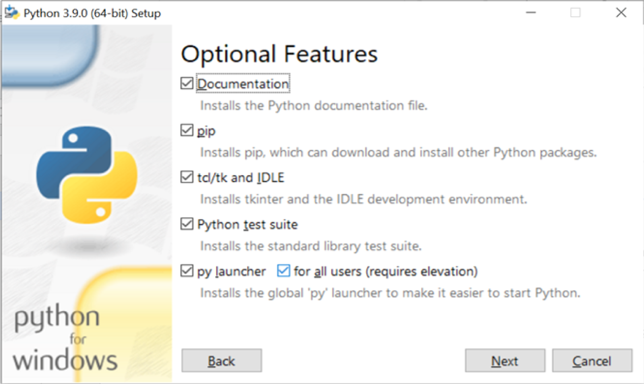
For each option, we have:

• Documentation: Will download the documentation of the Python version you are installing. All this information is also available on the Python documentation page, so it is unnecessary.
• Pip: Pip is a tool that helps to fetch packages for Python. When you install Python, you only have the standard library available, so you need a package manager to install specific libraries. Pip is the official supported one. We will discuss different package managers in later posts.
• IDLE: This stands for Integrated Development Learning Environment. This function will install the "tkinter" toolkit, a Python default GUI (Graphical User Interface) package.
• Python test suite: This installs all the standard libraries for Python application testing. The test package is meant for internal use by Python only. It is documented for the benefit of the core developers of Python. Any use of this package outside of Python’s standard library is discouraged.
• Py launcher: Enables you to launch Python CLI (Command Line Interface) like command prompt or Windows shell.
• For all users: Same as the normal installer, it allows you to install the Python launcher for all system users.

After clicking next, we will have the last customizable screen, where developers can check all the additional features. Some may have already been checked depending on the choices made before.

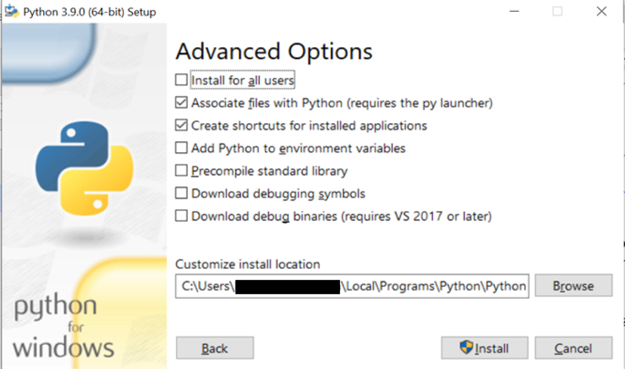
• Install for all users: This installs the Python launcher for all the users in your system.
• Associate files with Python: This option will link all the files Python extensions like .py, .pyd, .pyc or .pyo with the Python launcher or editor.
• Create a shortcut for installed applications: It will automatically create a shortcut for applications on the Desktop.
• Add Python to environment variables: PATH is an environment variable that holds values related to the current user and operating system. It specifies the directories in which executable programs are located. So when you type Python, Windows gets its executable from PATH. Hence, you won't need to type the whole path to the file on the command line.

The last three options tell the Python installation wizard to install all the debug symbols and binaries along with the bytecode of all the standard libraries, which we will be using with our programs. Finally, we can change the location of the Python installation directory. The location you specify will be added to the environmental variable of our Windows operating system.

---

Installing it lets you go to your terminal and execute a Python script. Assuming that you know how to deploy and work with the terminal (command tool) in your computer, once you have an interpreter installed, you can run a Python code by going to the folder where the py file is stored (from the terminal), and run:

python my_script.py

Being 'my_script' the name of our dummy code. This will instruct the Python interpreter stored on your computer to read that file. Assuming that the code obeys the grammatical rules of Python and the instructions in the code have to provide an output, this will appear in the terminal window. Again, this is an example of a very simple code. Some codes also require input from the user, and for that, we will need further tools.

Installing Python (MacOS)

For Mac users, there are different ways to install Python: by going to the official Python page and installing it directly from the page or using the Anaconda package (which we will show in another post).

Downloading the installer:

Most recent versions of Mac computers no longer have a pre-installed version of Python, and if your computer is brand new, most likely, it does not have it installed. Either way, it is always good practice to check if we have a previous version of Python installed so the packages do not clash.

To see if you have installed any Python version, launch the terminal of your computer by:

1. Searching for it in the Applications folder.
2. Command + Space bar and typing "Terminal"

and type python --version in it and hit Enter. If it’s not installed, you will see command not found: python. If installed, it will show you which version you have installed. Alternatively, you can type Python, and the terminal will automatically enter a Python running script, showing the Python version you have and the date of its release.

If Python is not installed, you can then use the installer. When you open the official page with your Mac, it automatically gives you the option for the latest version of the MacOS operating system.

Run the installer and follow the instructions. When you reach the installation type section, ensure enough space in your disk to install this package.

If you have partitions in your disk and want to change the installation location, you can select this by clicking the Change Install Location and choosing the disk you want. If not, click Install. The installation might take 5 to 10 minutes, depending on your internet connectivity. When the installer is finished copying files, double-click the Install Certificates command in the finder window to ensure your SSL root certificates are updated.

Restart your terminal (you can close it and open it in a new window) and repeat the process of checking the Python version. It should show you the version you have just installed.

Setting up environments

Global and Virtual environments

Now that we have installed Python, we mentioned that it comes with certain pre-installed basic libraries. But what happens when you want to use Python for a specific task and need to install additional packages? For this, Python has enabled pip, a recursive acronym for "Pip Installs Packages" or "Pip Installs Python", as its package manager to automate installation, update, and package removal.

However, installing new packages directly into the download of Python can have difficult consequences. This Python we just installed is the Global environment. We mentioned that Python is an open-source interpreted programming language that goes through constant updates. For this reason, newer libraries developed on different Python versions often conflict with libraries without the same updates, and error messages start to pop up.

Dmitriy Zub, Dec 22, 2021. Python Virtual Environments tutorial using Virtualenv and Poetry. Place of publication: SerpApi. Available here.

This image is a beautiful, chaotic example of what happens to your global environment when we do not have order in the different paths and versions of new packages.

To avoid this, a good practice when using Python is to use virtual environments. This environment allows for isolating package dependencies so they do not clash. For example, you may have two projects, one for computer vision and another for Natural Language Processing (NLP). Both of them use similar libraries but in different versions of Python. We can not install both versions system-wide, but we can create isolated environments for each project.

There are different ways to build Python environments:

Python environments (venv):

For this type of environment, the only requirement for your computer is to have a version of Python installed on it. venv is a Python module that supports lightweight virtual environments.

For this type of environment, you need to be familiar with how the terminal works, how you can move from one folder to another, and the Python versions you have installed. If you are unfamiliar with these requirements, please refer to the How to use Anaconda section.

From Python 3.3 onwards, venv should be included in the commands available. To create a virtual environment with this, please open your terminal:

macOS

To enter the terminal, you can search it directly from the Launchpad or application folder. Type Command + Space bar and type terminal for a shortcut. First, we must ensure you are in the folder where you want to save the environment. When you open the terminal, you should see only your user name:

For this example, I am going to access my Documents folder. You can access whatever folder you wish to save your environment on.

python -m venv [name of the environment]

Inside of the brackets, you can change it to whatever name you want. Just make sure that the name of the environment is something easy to remember, or write it down somewhere. The name should also follow the terminal rules: if you are going to name something with more than one word, you need to hyphenate the words with an underscore (_).

• Example: python -m venv example_environment.

The way you activate it is while inside the folder where you created the environment, call source [name of the environment]/bin/activate. The name in front of the dollar sign should change to the name of the environment you are currently in.

• Example:

WINDOWS OS

For the Windows OS you also need to have previously installed Python.

If you have Python already in your Path variables, you can just use the same arguments as the macOS instructions.

• Example: python -m venv example_environment

Please note that the same rules apply to Windows, so make sure to name the environment something unique and easy to remember, and also select the correct folder for your environment.

Conda environments

Another way to create environments in Python is to use the Anaconda distribution. For this, we have two options: we can download Anaconda from the official distribution or a more light version of Anaconda called Miniconda.

If you go for the Anaconda version:

macOS

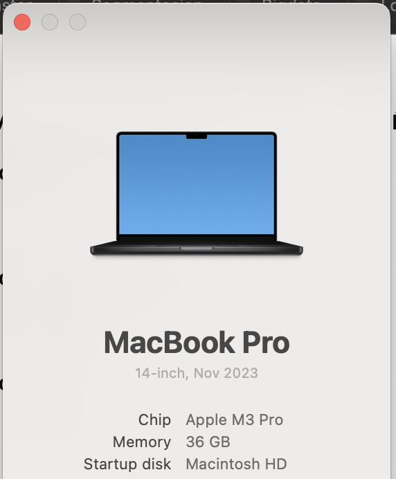
If you go to the official Anaconda page (https://www.anaconda.com/download#downloads), you will see the Download button for your OS. If you are using macOS, it is also important to know if your hardware settings are an Intel chip or an M1/M2/M3 chip.

You can check this by going to the Apple at the top left corner of your screen and clicking on About this Mac.

This should prompt a Window that will say the chip your computer has:

Go back to the Downloads page on Anaconda and choose the right setting for your computer.

Once the package is done loading, you can choose the predetermined installation and click install. If your terminal was opened, please relaunch it, you will now be able to see the pre fix in your user name as (base). Which means that you are in the base or root environment. We explain this later on.

It goes from:

To look something like this:

For Windows users:

For Windows, there is only one universal installer, so it does not matter the version of Windows that you are using. It is only important to know that it is only available for the 64-bit version. If your computer is a 32-bit, please look into the Anaconda archive (https://docs.anaconda.com/free/anaconda/install/old-os/).

Follow the installation process. Same as with the Python installation, this installer is going to ask you if you want to add this software to your path variables. If you are not sure or do not understand fully what path does, do not activate this function. We can change it later on if you need it.

Installing Miniconda

Graphical installer:

macOS

You must download the Miniconda installer from the official page (https://docs.anaconda.com/free/miniconda/). From here, you can choose the Intel or the M1/2/3 chip version and the bash or pkg versions. We strongly recommend using the bash version since the pkg may skip the "Destination select" process, failing the installation.

bash

• Once you download the document, locate where it is stored (it is most likely in the Downloads folder).
• Go to a new terminal in your computer (Command + Space bar type terminal + Enter)
• Go into the folder where you have the bash file stored (Ej. cd Downloads); you can verify it is there by running ls.
• This is an optional step, but we recommend verifying the download to ensure everything will run correctly. In your terminal run shasum -a 256 filename replacing filename with the downloaded file name. If it does not raise any error, follow the next step.
• Run bash <conda-installer-name>-latest-MacOSX-x86_64.sh. Replace the <conda-installer-name> with the downloaded file's name.
• Once the process is finished, please close and reopen your terminal (Command + q to close/reboot the program completely. You can see if this was successful by clicking Command + tab. It should show you all the applications you have opened. Make sure that the terminal does not show there).
• To verify the installation, open a terminal window and run conda list. If you installed everything correctly, a list of all the installed packages should appear.

Windows

For Windows, you can just download the .exe file and run it. In case you want to install it directly from the command line, you can run the following code:

curl https://repo.anaconda.com/miniconda/Miniconda3-latest-Windows-x86_64.exe -o miniconda.exe

The curl command allows the terminal to exchange data directly from another server, in this case, it is making an HTTP request, just like a web browser. If the request fails, make sure that your internet connection is stable. Once the download is complete, type:

start /wait "" miniconda.exe /S

This will start the installation process. Afterward, you can run del miniconda.exe to delete the executable file.

After installing, close the terminal and open the "Anaconda Prompt (miniconda3)" to use miniconda.

How to enable GPU support with TensorFlow (Windows) (For High Holborn only)

This article will guide you through how to enable GPU computing for Tensorflow on High Holborn DELL PCs.
The current version of Cuda Toolkit installed on DELL PCs is v12.2, but because the cuDNN library isn’t pre-installed, each student wanting to use tensorflow with GPU enabled should create a new environment using Anaconda Prompt and follow these steps:

1. Create a new conda enviroment with a Python version ranging from 3.7 to 3.10
   conda create -n ENV_NAME python=3.10
2. Install tensorflow 2.10
   pip install tensorflow==2.10.0
3. Install cuDNN from conda forge
   conda install -c conda-forge cudnn=8.1.0
4. Test tensorflow
   python -c "import tensorflow as tf; print(tf.config.list_physical_devices('GPU'))"
If the last command returned:
[PhysicalDevice(name='/physical_device:GPU:0', device_type='GPU')]
Tensorflow is ready to go!

How to enable GPU support with TensorFlow (macOS)

If you are using one of the laptops on loan of the CCI, or have a Macbook of your own with an M1/M2/M3 chip, here is what you can do to make full use of this chip with Tensorflow.

Requirements:

• macOS 12.0 or later
• Python 3.8 or later
• Mac with M1/M2/M3 chip

Steps:

1. Go to your terminal and create a new virtual environment with

conda create -n ENV_NAME python=PYTHON_VERSION -y

For this line of code, instead of ENV_NAME you can add any other name. Just make sure there is no other environment with the same name by typing conda env list in your terminal. That should show you a list with the names of all the other environments that computer has. For the Python version, you can choose any version later than 3.8. For more info about Python versions, see the Python language wiki page.

2. Go into your environment by typing

conda ENV_NAME activate

3. Check the version of Tensorflow you need before installing it.

   • For Tensorflow 2.13 or LATER: python -m pip install tensorflow
   • For Tensorflow 2.12 or EARLIER python -m pip install tensorflow-macos

4. Now we need to install the tensorflow-metal plug-in, running the line:

python -m pip install tensorflow-metal

For more info about the metal plig-in for mac, please read: Apple-Metal

5. After the installation is complete, you can copy and run the next python lines.

import tensorflow as tf

print(f"Tensor Flow Version: {tf.__version__}")
print()
print(f"Python {sys.version}")

gpu = len(tf.config.list_physical_devices('GPU'))>0
print("GPU is", "available" if gpu else "NOT AVAILABLE")

The output should be the tensorflow and python version you installed, and if everything is correct, the final message will be that the GPU is available

Enable GPU support with Pytorch (macOS)

This tutorial is to enable the use of the GPU in the Macbooks available on the lockers. All of these computers have Python and Anaconda already installed, so if you are using your personal computer, make sure that you have that installed before starting this tutorial. Please take a look at the other wiki pages about installing both Python and Anaconda.

Requirements:

• Macbook with M1/M2/M3 chip available
• macOS 12.3 or later
• Python 3.8 or later
• Package manager such as Anaconda or pip.

Steps:

1. Open your terminal and create a new virtual environment with:

   conda create -n ENV_NAME python=PYTHON_VERSION -y

Replace ENV_NAME with the name of your environment. The name can be anything, just make sure that it is not being used already. You can check that by typing conda env list. Also, remember that the name has to be a single compound word, and no spaces, for example, my_environment, or pytorch_env are good. my environment and pytorch env are not.

For the Python version, check for the best version for all the other libraries you need for your project.

2. Activate your environment from your terminal with:

   conda activate ENV_NAME

3. Install PyTorch by running:

   pip3 install --pre torch torchvision torchaudio --index-url https://download.pytorch.org/whl/nightly/cpu

This will install Pytorch and all the important dependencies in that library, like torchvision and torchaudio (to this, you can additionally add torchtext).

4. Test your install by running the next Python code. The output of it should be tensor([1.], device='mps:0')

import torch
if torch.backends.mps.is_available():
    mps_device = torch.device("mps")
    x = torch.ones(1, device=mps_device)
    print (x)
else:
    print ("MPS device not found.")

5. Additional information: Pytorch has a lot of documentation of its different modules, but a very useful one is to know how to assign hardware as a backend (this means it helps you set up and run operations on the GPU). For the mps device, we assign it like in the next example:

# Check that MPS is available
if not torch.backends.mps.is_available():
    if not torch.backends.mps.is_built():
        print("MPS not available because the current PyTorch install was not "
              "built with MPS enabled.")
    else:
        print("MPS not available because the current MacOS version is not 12.3+ "
              "and/or you do not have an MPS-enabled device on this machine.")

else:
    mps_device = torch.device("mps")

    # Create a Tensor directly on the mps device
    x = torch.ones(5, device=mps_device)
    # Or
    x = torch.ones(5, device="mps")

    # Any operation happens on the GPU
    y = x * 2

    # Move your model to mps just like any other device
    model = YourFavoriteNet()
    model.to(mps_device)

    # Now every call runs on the GPU
    pred = model(x)

How to install CUDA Toolkit on your personal Windows PC

What is CUDA Toolkit and why do you need it?

In simple words CUDA Toolkit allows you to develop software capable of utilising GPUs. CUDA Toolkit allows you to use CUDA runtime library for your C/C++ projects. CUDA Toolkit allows you to enable GPU acceleration for some useful Python libraries like Tensorflow, Numba, CuPy.

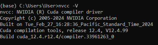
Checking if you already have CUDA Toolkit installed.

Open CLI and run nvcc -V command. If you get a similar output you already have CUDA Toolkit version installed. You might need to install additional software like cuDNN for Tensorflow.

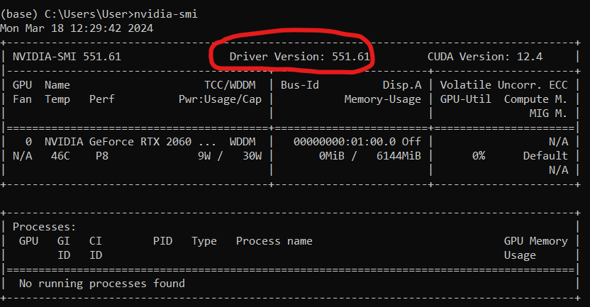
Checking your NVIDIA Driver version

Open CLI and run nvidia-smi command. If the command returns an error, you don't have an NVIDIA Driver installed. The highlighted number is your exact NVIDIA Driver version.

Note: CUDA version number in the table represents the latest CUDA Toolkit version your current NVIDIA Driver supports. It does not represent your currently installed CUDA Toolkit version, or even if you have it installed.

Installing NVIDIA Driver

Even if you have an NVIDIA Driver installed, you might need to upgrade your current version, to access the newest CUDA version.

1. Open following link in your browser:
https://www.nvidia.co.uk/Download/index.aspx?lang=en-uk
2. Fill out the dropdown list on the website.
3. In case you don’t know exact name of your GPU:

• In the Windows search bar enter “Device Manager”.
• Click the arrow next to Display adapters.
• Find the GPU starting with NVIDIA, this is your GPU.

Download the driver.

Follow the installation instructions.

Reboot your computer.

Open CLI and run nvidia-smi command. If the driver version changed, you successfully updated your NVIDIA Driver version.

Installing CUDA Toolkit

1. Open following link in your browser:
https://developer.nvidia.com/cuda-downloads
2. Follow the instructions
3. Select exe (network or local) and click the download button
4. Follow the installer instructions

• Installer will try to install GeForce Experience software. To disable it, use the custom install option.

Reboot your PC.

Open CLI and run nvcc -V command. If you get an output containing the version of the CUDA Toolkit you selected, you successfully installed CUDA Toolkit on your computer.

Note: If you execute nvcc -V command from the Anaconda Prompt CLI from the environment with pytorch library, it might display CUDA Toolkit version installed with pytorch instead of the one installed in your system.

Installing cuDNN library

This is an additional library you need to install to enable GPU computation in tensorflow.

1. Open following link in your browser:
https://developer.nvidia.com/rdp/cudnn-archive
2. Select the desired cuDNN version.
3. Follow the instructions
4. Select exe(network) and click the download button
5. Follow the installer instructions

Installing a different version of CUDA Toolkit

In some cases you will need to install older versions of both CUDA Toolkit and cuDNN.
Example: Repository for StyleGAN 2 requires you to have tensorflow 1.15. This version of tensorflow does not support newer versions of CUDA Toolkit.

1. Before proceeding, be sure that the configuration you want to install is supported. To do this consult CUDA Toolkit and cuDNN compatibility matrices:
https://docs.nvidia.com/deploy/cuda-compatibility/index.html#binary-compatibility__table-toolkit-driver
https://docs.nvidia.com/deeplearning/cudnn/archives/cudnn-801-preview/cudnn-support-matrix/index.html
https://docs.nvidia.com/deeplearning/cudnn/reference/support-matrix.html
2. Completely uninstall CUDA Toolkit. They can be found in
   Windows Settings > Apps > Apps & features
3. If your current NVIDIA Driver version supports the desired CUDA Toolkit version, proceed to step 5.
4. This step is very risky!
If your current NVIDIA Driver version does not support the desired CUDA version, you would have to uninstall your current Nvidia Driver and install the appropriate version.
This can be done in:
Windows Settings > Apps > Apps & features
5. Install the desired CUDA Toolkit from here https://developer.nvidia.com/cuda-toolkit-archive.
6. Install the desired cuDNN version.

How to register an account on JupyterHub

What is JupyterHub?

JupyterHub is a service we are trialing to allow students and staff to have access to GPU computing anywhere in UAL.

All you have to do is register your account and be connected to UAL-WiFi network.

To acess it, simply click on this link: https://jupyterdv.arts.ac.uk

The serivce itself is very simular to Jupyter Notebook and Jupyter Lab, but it's on the cloud, so you don't have to worry about limitations of your current personal PC or laptop.

The current configuration has multiple nodes with 16GB NVIADIA T4 GPU.

The service supports conda and venv for python environment managment.

If you ever used cloud computing platforms like Google Colab or Paperspace Gradient, this service will be very familiar.

Brief On Boarding

If JupyterHub is working correctly and you are not signed in, the landing page should look like this: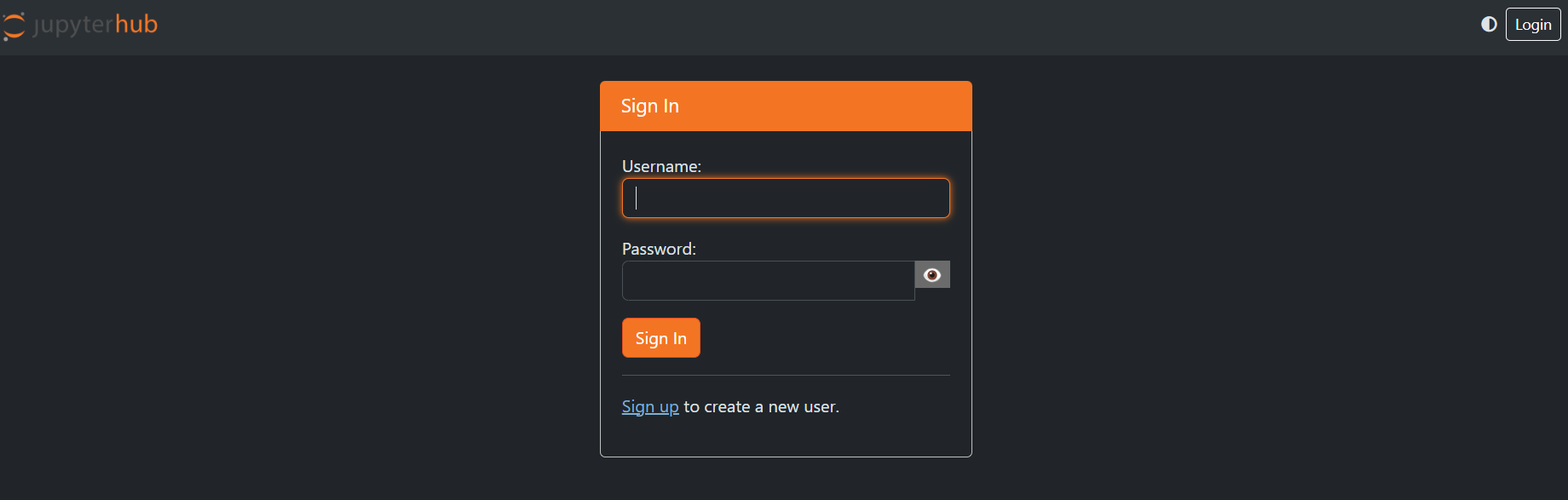

If you have an account, input your username and password to log in.

NOTE: UAL account is not the same as the JupyterHub account. If you never used this service, you need to create a new account.

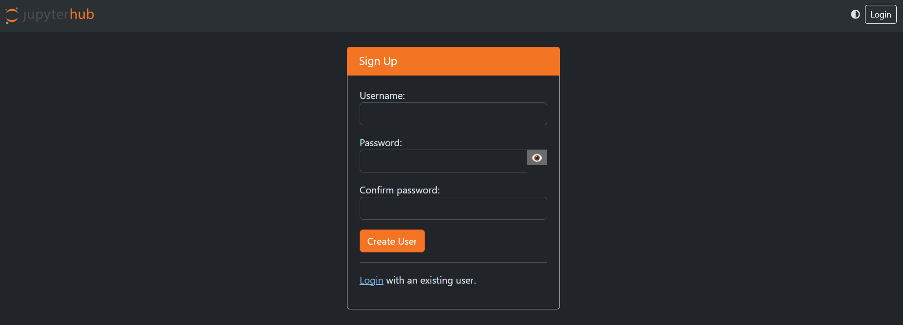
If you don't have an account. Press Sign Up button.

You will be prompted to input your new username and password. Do this.

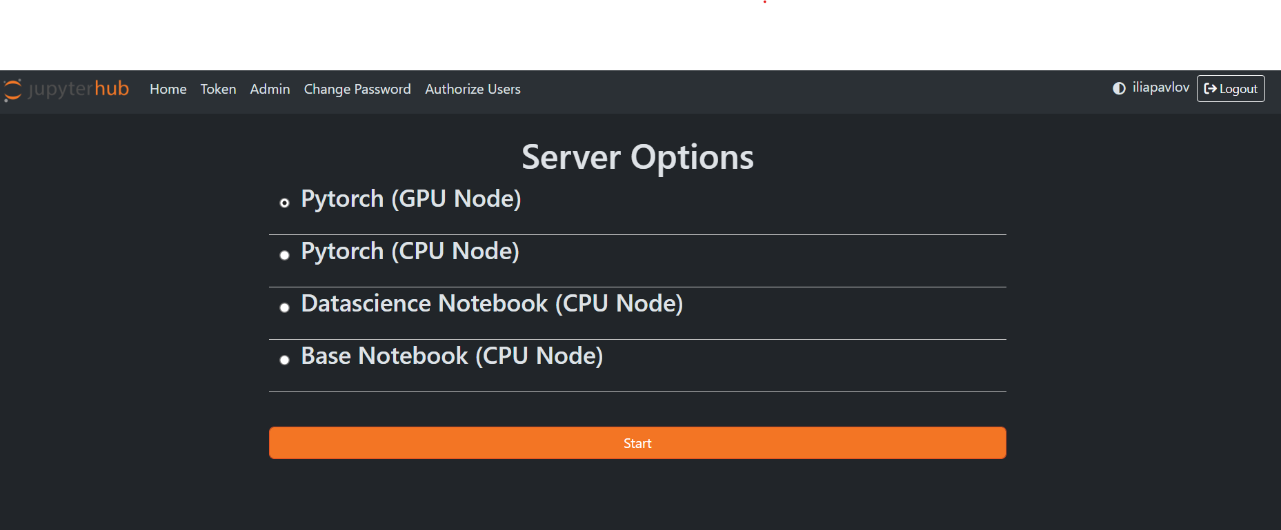
After creating your new account and singing in you should see this page. Select the appropriate option for your project and enjoy!

Simple PyTorch Project

Overview

This guide will walk you through a very simple PyTorch training pipeline. Accompanying code for this article can be found here:
https://git.arts.ac.uk/ipavlov/WikiMisc/blob/main/SimpleCNN.ipynb

Loading Libraries

Every Python project starts by loading all the relevant libraries. In our case, the code for that is:

import torch
from glob import glob
import cv2
import albumentations
from albumentations.pytorch import ToTensorV2
from torch.utils.data import Dataset, DataLoader

Reading the Dataset

For this example, we will use the MNIST dataset, containing 70,000 images of handwritten digits from 0 to 9. The specific version of MNIST used in this example can be found here: https://www.kaggle.com/datasets/alexanderyyy/mnist-png
Download the dataset and unpack it in the same directory your Jupyter Notebook is located. The unpacked dataset will consist of train and test folders containing images for model training and evaluation. Both test and train folders will have 10 sub-folders for each digit.

To train our model, we need to know the file names and labels of all images in the dataset. A simple way to do this is demonstrated in the code below:

def readMnist(folder):
    filenames = [] #List for image filenames
    labels = [] #List for image labels
    
    folderNameLen = len(folder) 
    
    #Reads all the filenames in a given folder recursively
    for filename in glob(folder + '/**/*.png', recursive=True): 
        filenames += [filename]
        #Get the label of the image from it’s filepath
        labels += [int(filename[folderNameLen:folderNameLen+1])]         
    return filenames, labels

trainFiles, trainLabels = readMnist('./mnist_png/train/')
testFiles, testLabels = readMnist('./mnist_png/test/')

Note: Different datasets will require different approaches.

Dataset Class

The Dataset class will provide necessary functionality to our training and evaluation pipeline, like loading images and labels, image transformations, and others.

class MnistDataset(Dataset):
    def __init__(self, filepaths, labels, transform):
        self.labels = labels
        self.filepaths = filepaths
        self.transform = transform
        
    def __len__(self):
        return len(self.labels)

    def __getitem__(self, idx):
        image = cv2.imread(self.filepaths[idx], 0)
        h,w = image.shape
            
        image = self.transform(image=image)["image"]/255.
        label = self.labels[idx]
        
        return image, label

# Usually transformations would include data augmentation tricks, 
# but for this example we will limit ourselves to just converting image data from
# NumPy array to PyTorch tensor.
transform = albumentations.Compose(
    [
        ToTensorV2()
    ]
)   

To allow for mini-batch use we need to introduce a DataLoader to our pipeline.

#Instantiate Dataset objects for train and test datasets.
trainDataset = MnistDataset(trainFiles, trainLabels, transform)
testDataset = MnistDataset(testFiles, testLabels, transform)

Model Class

Our model classifies the input images between 10 different classes. Below is the code for our simple convolutional neural network. The comments in the code will provide additional explanation.

class CNN(torch.nn.Module):
    # Inside of __init__ we define the structure of our neural network.
    # Thinks of this as a collection of all potential layers and modules 
    # that we will use during the feedforward process.
    def __init__(self):
        super().__init__() #Needed to initialize torch.nn.Module correctly
        
        # Our first convolutional block. torch.nn.Sequential is container
        # that will execute modules inside of it sequantialy. 
        # This convolutional block consists of a simple convolutional layer,
        # ReLU activation functions, and Max Pooling operation.
        self.conv1 = torch.nn.Sequential
          (torch.nn.Conv2d(
               in_channels=1,             
               out_channels=16,           
               kernel_size=5,             
               stride=1,                  
               padding=2,                 
           ),                             
           torch.nn.ReLU(),                     
           torch.nn.MaxPool2d(kernel_size=2),   
        )
        # Our second onvolutional block.
        self.conv2 = torch.nn.Sequential(        
           torch.nn.Conv2d(16, 32, 5, 1, 2),    
           torch.nn.ReLU(),                     
           torch.nn.MaxPool2d(2),               
        )
        # Fully connected layer that outputs 10 classes
        self.out = torch.nn.Linear(32 * 7 * 7, 10)
    
    # forward is a function that is used for feedforward operation of our model.
    # Input arguments are input data for our model. In this case x would be a batch of images from the MNIST dataset.
    # Inside of this function we apply modules we defined in __init__ to input images.
    def forward(self, x):
        x = self.conv1(x)
        x = self.conv2(x)
        #This line flattens tensors from 4 dimenstions to 2.
        x = torch.flatten(x, start_dim=1)     
        output = self.out(x)
        return output

# This line creates an object of our convolutional neural network class. 
# We use .cuda() to send our model to GPU.
model = CNN().cuda()

Training and Validation

Below is the code for our training and validation procedure.

#Here we define cross entropy loss functions, which we will use for loss calculation.
loss_fn = torch.nn.CrossEntropyLoss() 

#This is our optimizer algorithm. In this example we use Stochastic gradient descent
optimizer = torch.optim.SGD(model.parameters(), lr=0.001)

num_epochs = 25

#We will execute our training inside of a loop. Each iteration is a new epoch.
for epoch in range(num_epochs):
    print('Epoch:', epoch)
    
    running_loss = 0
    model = model.train() #sets our model to training mode.
    for i, data in enumerate(train_dataloader): #we will iterate over our dataloader to get batched data.
        x, y = data
        #Don't forget to send your images and labels to the same device as your model. In our case it's a GPU.
        x = x.cuda()
        y = y.cuda()

        #Resets gradients
        optimizer.zero_grad()
        #output of our CNN model
        outputs = model(x)
        #Here we calcualte loss values
        loss = loss_fn(outputs, y)
        
        loss.backward() #Backpropagation
        optimizer.step() #Backpropagation
        
        running_loss += loss.item()
    
    print(running_loss/len(train_dataloader)) #average training loss for current epoch
    
    model = model.eval() #sets our model to evaluation mode.
    test_acc = 0
    test_running_loss = 0
    for i, data in enumerate(test_dataloader):
        x, y = data
        x = x.cuda()
        y = y.cuda()

        outputs=model(x)
        loss = loss_fn(outputs, y)

        test_running_loss += loss.item()
        #We apply softmax here to get the probabilities for each class
        probs = torch.nn.functional.softmax(outputs, dim=1)
        #We select the highest probability as our final predication
        pred = torch.argmax(probs, dim=1)
        test_acc += torch.sum(pred == y)

    #Average evaluation loss and evaluation accuracy for this epoch
    print(test_running_loss/len(testDataset), test_acc/len(testDataset))

Audio Files with Librosa

Code and audio for this article can be found here:
https://git.arts.ac.uk/ipavlov/WikiMisc/blob/main/AudioProcessing.ipynb
Documentaion for Librosa can be found here:
https://librosa.org/doc/main/index.html

Loading audio files

Librosa is a Python libray created for working with audio data. It's both easy to understand and has an extensive feuture list.
By default Librosa supports all the popular audio file extensions, like WAV, OGG, MP3, and FLAC.

import librosa
import librosa.display

filename = librosa.ex('trumpet') #Loads sample audio file
y, sr = librosa.load(filename)

y — is a NumPy matrix that contains audio time series. If audio file is mono it will be one-dimensional vector, if audio file is stereo it will be two-dimensional, and so on.
sr — is audio file's sampling rate.

Playing audio in Jupyter notebook

Using the code bellow you will be able to play audio inside of your notebook. The player is very basic, but will be enough for simpler projects.

from IPython.display import Audio

Audio(data=y, rate=sr)

Vizualising audio files

To vizualise our audio files we can use Matplotlib.

import matplotlib.pyplot as plt

plt.figure(figsize=(12, 4))
librosa.display.waveshow(y, sr=sr) #This functions will dipslay audio file's waveform.
plt.show()

You can use code bellow to vizualize audio file's spectrogram. Please refer to Librosa's documantion for explanation for each function used in the code bellow: https://librosa.org/doc/main/index.html

fig, ax = plt.subplots()

S = librosa.feature.melspectrogram(y=y, sr=sr, n_mels=128,
                                    fmax=8000)

S_dB = librosa.power_to_db(S, ref=np.max) 
img = librosa.display.specshow(S_dB, x_axis='time',
                         y_axis='mel', sr=sr,
                         fmax=8000, ax=ax)
fig.colorbar(img, ax=ax, format='%+2.0f dB')
ax.set(title='Mel-frequency spectrogram')

Working with multiple audio files

You can work multiple audio files. Just assign the time series for each file to a different variable or create a list of audio time series.
The code bellow looks at all .wav files in a given folder.

from glob import glob

audio_filepaths = []

for filename in glob('./audio/*.wav'): 
    audio_filepaths += [filename]
    
audio_filepaths

Often times for AI&ML applications audio data needs to be of uniform length. To do this we can pad them.

padded_audio_files = []

max_allowed_length = 32000

for audio_filepath in audio_filepaths:

    y_voice, sr_voice = librosa.load(audio_filepath)
    
    if len(y_voice) > max_allowed_length:
        raise ValueError("data length cannot exceed padding length.")
    elif len(y_voice) < max_allowed_length:
        embedded_data = np.zeros(max_allowed_length)
        offset = max_allowed_length - len(y_voice)
        embedded_data[offset:offset+len(y_voice)] = y_voice
    elif len(y_voice) == max_allowed_length:
        embedded_data = y_voice
    
    padded_audio_files += [embedded_data]
    
padded_audio_files = np.array(padded_audio_files)

padded_audio_files.shape

You can also append multiple audio files together. Let's do it with our padded files.

long_number = padded_audio_files.flatten()
long_number.shape

The waveform of a new audio will look like this:

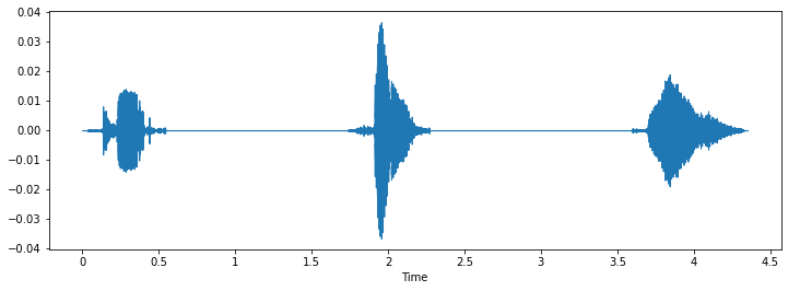
Note: Keep track of audio file shapes, espcially along the 2nd axis.

Advanced Audio Analysis

Librosa has a wide range of tools for audio analyses. Some examples are included bellow.
Short-time Fourier transform:

S = np.abs(librosa.stft(y))

S.shape

Decibel analysis:

D = librosa.amplitude_to_db(librosa.stft(y), ref=np.max)

D.shape

Spectral flux:

#This code was taken from here: https://librosa.org/doc/main/generated/librosa.onset.onset_strength.html
S = np.abs(librosa.stft(y))
times = librosa.times_like(S)
fig, ax = plt.subplots(nrows=2, sharex=True)
librosa.display.specshow(librosa.amplitude_to_db(S, ref=np.max),
                         y_axis='log', x_axis='time', ax=ax[0])
ax[0].set(title='Power spectrogram')
ax[0].label_outer()


onset_env = librosa.onset.onset_strength(y=y, sr=sr)
ax[1].plot(times, 2 + onset_env / onset_env.max(), alpha=0.8,
           label='Mean (mel)')

onset_env = librosa.onset.onset_strength(y=y, sr=sr,
                                         aggregate=np.median,
                                         fmax=8000, n_mels=256)
ax[1].plot(times, 1 + onset_env / onset_env.max(), alpha=0.8,
           label='Median (custom mel)')

C = np.abs(librosa.cqt(y=y, sr=sr))
onset_env = librosa.onset.onset_strength(sr=sr, S=librosa.amplitude_to_db(C, ref=np.max))
ax[1].plot(times, onset_env / onset_env.max(), alpha=0.8,
         label='Mean (CQT)')
ax[1].legend()
ax[1].set(ylabel='Normalized strength', yticks=[])

# Filters As with all Python libraries, to unlock the full potential of librosa they need to be used with other libraries. The code bellow shows you how to apply a butter filter to audio signal, with a help of SciPy. ```python scipy.signal.butter

fig, ax = plt.subplots(nrows=2, figsize=(12, 4), constrained_layout=True)

ax[0].set(title='Normal waveform')

librosa.display.waveshow(y, sr=sr, ax=ax[0])

sos = signal.butter(17, 150, 'hp', fs=1000, output='sos') filtered = signal.sosfilt(sos, y)

ax[1].set(title='Filtered waveform')

librosa.display.waveshow(filtered, sr=sr, ax=ax[1])

filtered = filtered - 0.25 # Hearing protection

<img src="https://github.com/locsor/imagesForWiki/blob/main/14.png?raw=true">

How to configure Weights & Biases for you ML project

What is Weights & Biases?

Weights & Biases (wandb from now on) is a platform for AI/ML development. A set of tools it provides can help you keep track of your model's training. This can be very useful if you want to check on how's your model training since you can access wandb remotly from your phone or home computer.

wandb set up

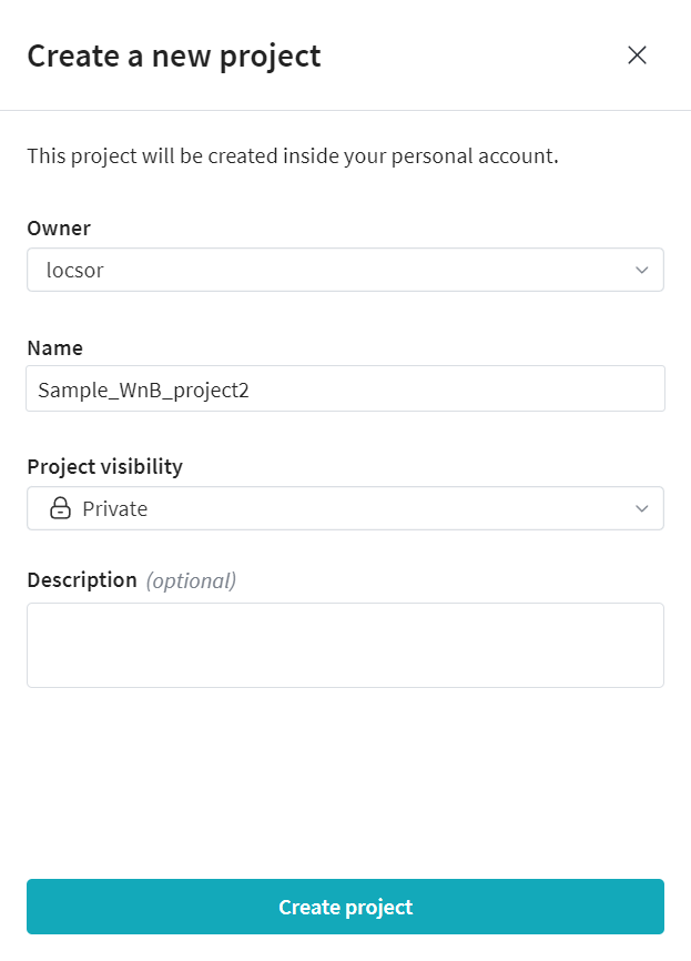
1. Create an account on wandb website.
2. Create a new project and set it's visibility.
   
   
3. Activate your Python enviroment.
4. Install wandb package from PyPi:
   pip install wandb
5. Login into your wandb account from console:
   wandb login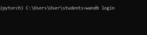

How to use wandb in your AI/ML project

The simplest use case for wandb is to use it to track your training progress. You can monitor training and validation loss values, test accuracy, and even see what data is being fed into your model during training and validation.

You can do this in four simple steps:

1. Import wandb library
2. Initialize wandb process with your project name, you can specify details abouth the training run, like batch size and learning rate.
3. Log the training information after every epoch.
4. Stop the process after training is finished.

You can refer to this block of code for step 2-4.

num_epochs = 25

if wandb and wandb.run is None:
    experiment_dict = {}
    experiment_dict['batch_size']=batch_size
    experiment_dict["learning_rate"]=learning_reate
    experiment_dict["epochs"]=num_epochs
    
    wandb_run = wandb.init(config=experiment_dict, resume=False,
                           project="Sample_WnB_project",
                           name="Test Run")

#We will execute our training inside of a loop. Each iteration is a new epoch.
for epoch in range(num_epochs):
    print('Epoch:', epoch)
    
    total_train_loss, model, optimizer = train(model, optimizer, loss_fn, train_dataloader)
    
    train_loss = total_train_loss/len(train_dataloader)
    
    print('Train loss: ', train_loss) #average training loss for current epoch
    
    total_test_loss, total_test_acc = evaluate(model, test_dataloader, loss_fn)
    
    test_loss = total_test_loss/len(testDataset)
    test_acc = total_test_acc/len(testDataset)
    
    #Average evaluation loss and evaluation accuracy for this epoch
    print('Test loss: ', test_loss)
    print('Test accuracy: ', test_acc)
    
    wandb.log({"acc": test_acc, "train_loss": train_loss, "test_loss": test_loss})
    
wandb.finish()

You can get the full code from: https://git.arts.ac.uk/ipavlov/WikiMisc/blob/main/SimpleCNN_tweak.ipynb
Data can be found here

Dataset Augmentaion

This article will cover how you can increase the size of your original dataset with the help of data augmentation. Data augmentaion is a practice of altering samples in your dataset, making them distinct enough from the original sample to be considered a new sample, and keeping alterations small enough to keep them recognizable as a part of the dataset's original data domain.
Examples: Adding slight noise to audio samples and mirroring images.

Image augmentaion

The simplest way to add data augmentaion to your training pipeline is to use Albumentations library.

Starting from the most basic ones, here are some augmentaion tricks you can use:

• Original image:
  

  image = Image.open("testImg.jpg")
  image_np = np.array(image)
  

• Image flipping or mirroring:
  

  transform = A.Compose([A.HorizontalFlip(p=1.0)])
  transformed_image = transform(image=image_np)["image"]
  

  
  

  transform = A.Compose([A.VerticalFlip(p=1.0)])
  transformed_image = transform(image=image_np)["image"]
  

• Image rotation:
  

  transform = A.Compose([A.Rotate(p=1.0, limit=45, border_mode=0)])
  transformed_image = transform(image=image_np)["image"]
  

• HSV Jitter:
  

  transform = A.Compose([A.ColorJitter(p=1.0)])
  transformed_image = transform(image=image_np)["image"]
  

• Gaussian Noise:
  

  transform = A.Compose([A.GaussNoise(p=1.0, var_limit=(1000.0, 5000.0))])
  transformed_image = transform(image=image_np)["image"]
  

Augmentaions almost always combined with each other:

  transform = A.Compose([
      A.HorizontalFlip(p=1.0),
      A.VerticalFlip(p=1.0),
      A.Rotate(p=1.0, limit=45, border_mode=0),
      A.RandomBrightnessContrast(p=1.0, brightness_limit=(0.15,0.25)),
      A.ColorJitter(p=1.0),
      A.GaussNoise(p=1.0, var_limit=(1000.0, 2000.0),),
  ])
  transformed_image = transform(image=image_np)["image"]

Above is an extremecase of image augmentaion, we still want to keep the resulting images as close to the original data distribution as possible:

  transform = A.Compose([
      A.HorizontalFlip(p=0.5),
      A.Rotate(p=0.5, limit=15, border_mode=0),
      A.RandomBrightnessContrast(p=0.5, brightness_limit=(-0.1,0.1)),
      A.ColorJitter(p=0.5),
      A.GaussNoise(p=0.5, var_limit=(50.0, 250.0),),
  ])
  transformed_image = transform(image=image_np)["image"]

Further Reading

You can follow the links bellow for example use of Albumentaions library with popular AI/ML libraries.

• Tensorflow.
• PyTorch.