Audio Files with Librosa
Code and audio for this article can be found here:
https://git.arts.ac.uk/ipavlov/WikiMisc/blob/main/AudioProcessing.ipynb
Documentaion for Librosa can be found here:
https://librosa.org/doc/main/index.html
Loading audio files
Librosa is a Python libray created for working with audio data. It's both easy to understand and has an extensive feuture list.
By default Librosa supports all the popular audio file extensions, like WAV, OGG, MP3, and FLAC.
import librosa
import librosa.display

filename = librosa.ex('trumpet') #Loads sample audio file
y, sr = librosa.load(filename)
y — is a NumPy matrix that contains audio time series. If audio file is mono it will be one-dimensional vector, if audio file is stereo it will be two-dimensional, and so on.
sr — is audio file's sampling rate.
Playing audio in Jupyter notebook
Using the code bellow you will be able to play audio inside of your notebook. The player is very basic, but will be enough for simpler projects.
from IPython.display import Audio

Audio(data=y, rate=sr)
Vizualising audio files
To vizualise our audio files we can use Matplotlib.
import matplotlib.pyplot as plt

plt.figure(figsize=(12, 4))
librosa.display.waveshow(y, sr=sr) #This functions will dipslay audio file's waveform.
plt.show()

You can use code bellow to vizualize audio file's spectrogram. Please refer to Librosa's documantion for explanation for each function used in the code bellow: https://librosa.org/doc/main/index.html
fig, ax = plt.subplots()

S = librosa.feature.melspectrogram(y=y, sr=sr, n_mels=128,
                                    fmax=8000)

S_dB = librosa.power_to_db(S, ref=np.max)
img = librosa.display.specshow(S_dB, x_axis='time',
                         y_axis='mel', sr=sr,
                         fmax=8000, ax=ax)
fig.colorbar(img, ax=ax, format='%+2.0f dB')
ax.set(title='Mel-frequency spectrogram')

Working with multiple audio files
You can work multiple audio files. Just assign the time series for each file to a different variable or create a list of audio time series.
The code bellow looks at all .wav files in a given folder.
from glob import glob

audio_filepaths = []

for filename in glob('./audio/*.wav'):
    audio_filepaths += [filename]

audio_filepaths
Often times for AI&ML applications audio data needs to be of uniform length. To do this we can pad them.
padded_audio_files = []

max_allowed_length = 32000

for audio_filepath in audio_filepaths:

    y_voice, sr_voice = librosa.load(audio_filepath)

    if len(y_voice) > max_allowed_length:
        raise ValueError("data length cannot exceed padding length.")
    elif len(y_voice) < max_allowed_length:
        embedded_data = np.zeros(max_allowed_length)
        offset = max_allowed_length - len(y_voice)
        embedded_data[offset:offset+len(y_voice)] = y_voice
    elif len(y_voice) == max_allowed_length:
        embedded_data = y_voice

    padded_audio_files += [embedded_data]

padded_audio_files = np.array(padded_audio_files)

padded_audio_files.shape
You can also append multiple audio files together. Let's do it with our padded files.
long_number = padded_audio_files.flatten()
long_number.shape
The waveform of a new audio will look like this:
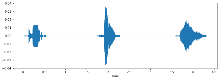
Note: Keep track of audio file shapes, espcially along the 2nd axis.
Advanced Audio Analysis
Librosa has a wide range of tools for audio analyses. Some examples are included bellow.
Short-time Fourier transform:
S = np.abs(librosa.stft(y))

S.shape
Decibel analysis:
D = librosa.amplitude_to_db(librosa.stft(y), ref=np.max)

D.shape
Spectral flux:
#This code was taken from here: https://librosa.org/doc/main/generated/librosa.onset.onset_strength.html
S = np.abs(librosa.stft(y))
times = librosa.times_like(S)
fig, ax = plt.subplots(nrows=2, sharex=True)
librosa.display.specshow(librosa.amplitude_to_db(S, ref=np.max),
                         y_axis='log', x_axis='time', ax=ax[0])
ax[0].set(title='Power spectrogram')
ax[0].label_outer()


onset_env = librosa.onset.onset_strength(y=y, sr=sr)
ax[1].plot(times, 2 + onset_env / onset_env.max(), alpha=0.8,
           label='Mean (mel)')

onset_env = librosa.onset.onset_strength(y=y, sr=sr,
                                         aggregate=np.median,
                                         fmax=8000, n_mels=256)
ax[1].plot(times, 1 + onset_env / onset_env.max(), alpha=0.8,
           label='Median (custom mel)')

C = np.abs(librosa.cqt(y=y, sr=sr))
onset_env = librosa.onset.onset_strength(sr=sr, S=librosa.amplitude_to_db(C, ref=np.max))
ax[1].plot(times, onset_env / onset_env.max(), alpha=0.8,
         label='Mean (CQT)')
ax[1].legend()
ax[1].set(ylabel='Normalized strength', yticks=[])

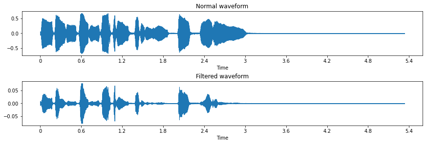
Filters
As with all Python libraries, to unlock the full potential of librosa they need to be used with other libraries. The code bellow shows you how to apply a butter filter to audio signal, with a help of SciPy.
scipy.signal.butter

fig, ax = plt.subplots(nrows=2, figsize=(12, 4), constrained_layout=True)

ax[0].set(title='Normal waveform')

librosa.display.waveshow(y, sr=sr, ax=ax[0])

sos = signal.butter(17, 150, 'hp', fs=1000, output='sos')
filtered = signal.sosfilt(sos, y)

ax[1].set(title='Filtered waveform')

librosa.display.waveshow(filtered, sr=sr, ax=ax[1])

filtered = filtered - 0.25 # Hearing protection